
Observables#
pianistpy.sigma_los(), pianistpy.sigma_los_aperture(), pianistpy.aperture_losvd(),
pianistpy.Aperture, pianistpy.LosTable
Observables are functions of a model. Given a model, losvd and aperture_losvd build the model’s
line-of-sight table (LosTable) at every call. For repeated requests on one model, build
LosTable(model) once. A LosTable tabulates the line-of-sight velocity distributions of the model, and every
observable accepts the LosTable in place of the model.
sigma = pp.sigma_los(model, [0.1, 1.0, 10.0])        # at projected radii

circle = pp.Aperture.circle(r_ape=1.0, r_off=0.0)
slit = pp.Aperture.rectangle(side_x=2.0, side_y=0.2, r_off=0.0, angle=0.0)
pp.sigma_los_aperture(model, circle)                 # averaged over an aperture
pp.sigma_los_aperture(model, slit)

table = pp.LosTable(model)                           # once, for many requests
pp.sigma_los(table, [0.1, 1.0, 10.0])
pp.sigma_los_aperture(table, circle)
pp.aperture_losvd(table, circle, [0.0, 0.1, 0.2])    # the distribution in the aperture
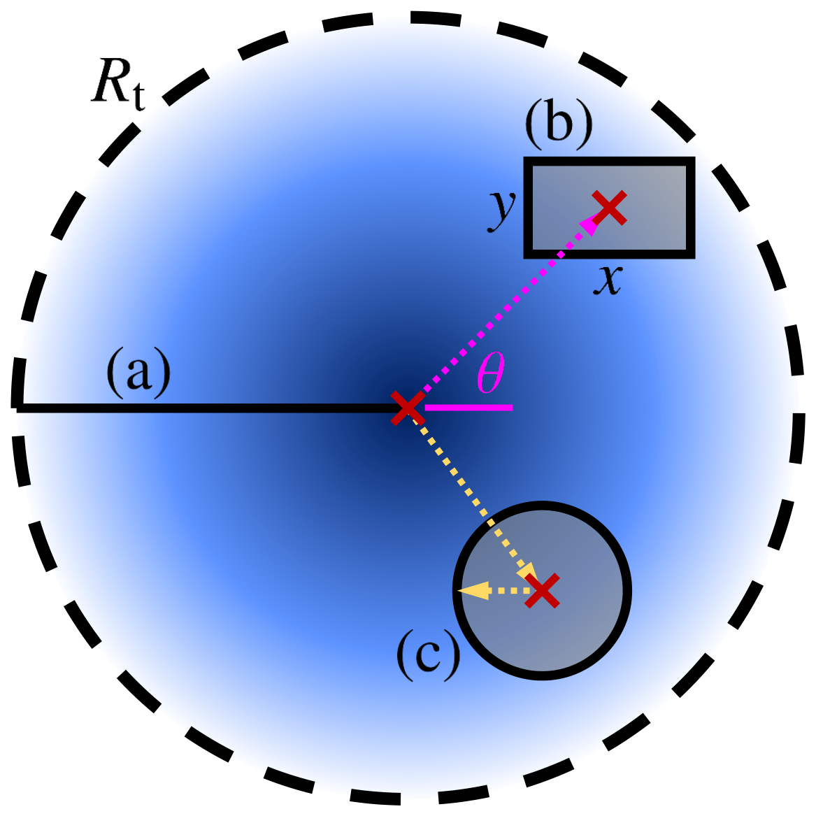
The projection configurations of a spherical system truncated at \(R_{\rm t}\) (dashed circle), from
Chiang+(2026d), Fig. 14. (a) The projected radial profile along the line of sight, as for a slit of negligible width.
(b) The average over a rectangular aperture of sides \(x\) and \(y\) (side_x, side_y), whose
center lies at the projected distance r_off from the center of the system, on a line at the angle
\(\theta\) (angle) to the rectangle’s \(x\) side, as for a slit of finite width. (c) The average
over a circular aperture, centered or offset, as for fiber-fed observations.#
An Aperture is a circle or a rectangle, centered or offset. A rectangle also takes an angle, in radians,
between the rectangle’s x axis and the line through the center of the model and the center of the rectangle.
sigma_los_aperture and aperture_losvd take the same Aperture object. sigma_r, sigma_t, losvd
and pdf_v also take a model or the model’s line-of-sight table as the first argument. The
Observables page of the API reference lists every call. The Gauss-Hermite
moments \(h_3\) and \(h_4\) of the line-of-sight velocity distribution have no top-level call. The inference
takes \(h_3\) and \(h_4\) as data (pianistpy.inference.Data).
ProjectedSampler draws pairs of projected radius and line-of-sight velocity on an annulus and, if given, in a
user-specified range of line-of-sight velocity. For every anisotropy model, the draw is conditioned exactly on the
velocity range. At each projected radius, the distribution of the projected radius is weighted by the share of the
line-of-sight velocity distribution inside the velocity range. The ranges and the drawn pairs are in the unit system
of the model or the line-of-sight table given to ProjectedSampler, as for the other observables. The attribute
validation of a ProjectedSampler is the validation report of the draw.
sampler = pp.ProjectedSampler(table, R_range=(0.1, 3.0), v_range=(-0.2, 0.3))
pairs = sampler.sample(1_000_000, seed=1)   # pairs.r_2d, pairs.v_los, pairs.mass
Observables over an aperture of any other shape can be estimated by Monte Carlo. Draw pairs with
ProjectedSampler on an annulus that encloses the aperture, give each pair a uniformly random position angle
(the model is spherical), and keep the pairs inside the aperture. Sums over the kept pairs, each with its mass
(pairs.mass), give the aperture’s mass, dispersion and velocity distribution, with a statistical error that
falls as the inverse square root of the number of pairs.
- Radial velocity dispersion (sigma_r)
- Tangential velocity dispersion (sigma_t)
- Line-of-sight velocity distribution (losvd)
- Line-of-sight velocity distribution in an aperture (aperture_losvd)
- Local velocity distribution (pdf_v)
- Line-of-sight table (LosTable)
- End-to-end differentiability
- Differentiable observables (Differentiable)